This guide covers the direct materials cost variance formula, how to break it into its price and quantity components, and a step-by-step walkthrough using a concrete pour scenario that mirrors what actually happens on commercial projects.
Key Takeaways
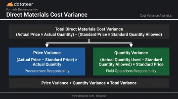
- Total direct materials cost variance = (Actual Quantity × Actual Price) – (Standard Quantity × Standard Price)
- It splits into two sub-variances: price variance (procurement) and quantity variance (field operations)
- Favorable = spent less than budgeted; unfavorable = spent more
- Construction-specific drivers include commodity swings, supply chain delays, change orders, and field waste
- Catching variance during the project — not at closeout — gives you time to act before margin is lost
What Is Direct Materials Cost Variance in Construction?
Direct materials cost variance is the dollar difference between what a construction firm expected to pay for materials (standard cost) and what it actually paid (actual cost), calculated as price per unit multiplied by quantity purchased or used.
Construction has no recurring production runs. Materials get bid at one price, procured at a different one, and consumed in the field at rates that shift with conditions — each stage introducing potential variance. A factory sets a standard cost and runs the same process thousands of times. A construction firm sets a project budget, then executes once under changing field conditions.
Two root causes drive any materials cost variance:
- Price variance — you paid more or less per unit than planned
- Quantity variance — you used more or fewer units than the scope required
The corrective actions point in completely different directions depending on which driver is responsible. Price variance leads you to procurement. Quantity variance leads you to the field — or back to the original estimate.
The Direct Materials Cost Variance Formula: Price, Quantity, and Total
The Master Formula
Total Direct Materials Cost Variance = (Actual Quantity × Actual Price) – (Standard Quantity × Standard Price)
A positive result means you spent more than budgeted — unfavorable. A negative result means you came in under budget — favorable. Remember: higher actual cost = positive number = unfavorable for margin.
Direct Materials Price Variance
Price Variance = (Actual Price – Standard Price) × Actual Quantity Purchased
This component isolates whether the firm paid more or less per unit, regardless of how much was used. It's calculated at the time of purchase, not consumption, because the cost locks in the moment the PO is executed.
In construction, price variance is driven by:
- Commodity market movements (steel indices, lumber futures, ready-mix pricing)
- Emergency procurement outside negotiated supplier agreements
- Geographic scarcity or regional shortages
- Fuel surcharges passed through by suppliers
AGC's June 2025 data shows fabricated structural metal for bridges up 22.5% year over year — the kind of swing that produces significant unfavorable price variances on steel-heavy scopes, no matter how carefully the field manages quantities.
Direct Materials Quantity Variance
Quantity Variance = (Actual Quantity Used – Standard Quantity Allowed) × Standard Price
This component isolates whether the project consumed more or fewer materials than the standard allows for the actual scope completed. Note: "standard quantity allowed" must reflect actual work completed (not the original budget scope).
Quantity variance in construction is driven by:
- Field waste and cutting loss (rebar offcuts, concrete overpouring)
- Design changes and rework
- Inaccurate quantity take-offs in the original estimate
- Theft or damage on site
Notice that standard price — not actual price — appears in the quantity variance formula by design. Using standard price isolates the quantity problem from the pricing problem, so each variance tells a clean story.
The two sub-variances sum to the total:
Price Variance + Quantity Variance = Total Direct Materials Cost Variance
How to Calculate Direct Materials Cost Variance: Step-by-Step
Here's how the calculation actually flows on a construction project, from setting the standard through reporting the result.
Step 1 – Establish the Standard Cost and Standard Quantity
Standard cost is the budgeted unit price for each material line item, set during estimating using current supplier quotes, historical averages, or published indices like BLS PPI. Standard quantity is the estimated material takeoff for the scope completed to date.
The critical rule: standard quantity must track against actual completed work, not the original budget. If 60% of the foundation is poured, the standard quantity allowed should reflect 60% of the total takeoff, not 100%.
Step 2 – Capture Actual Cost and Actual Quantity
- Actual cost per unit comes from purchase orders and supplier invoices in your ERP or accounting system
- Actual quantity used comes from field consumption reports, delivery receipts, and material tracking logs
A common gap: most firms have accurate PO data but poor visibility into actual field consumption. That gap means quantity variances go undetected until project closeout, when corrective action is no longer possible.
Step 3 – Calculate the Price Variance
Apply: (Actual Price – Standard Price) × Actual Quantity Purchased
A small per-unit gap of $3/CY on concrete, multiplied by 500 cubic yards, produces a $1,500 variance. Multiply that across multiple material lines and multiple project phases, and the total exposure adds up quickly. Track price variance at the line-item level, not just the project total, so early signals don't get buried.
Step 4 – Calculate the Quantity Variance
Apply: (Actual Quantity Used – Standard Quantity Allowed) × Standard Price
Using standard price here is deliberate. It keeps this variance clean, measuring only the quantity overrun or underrun at the originally budgeted rate.
Step 5 – Combine and Interpret the Total Variance
Add price variance + quantity variance = total direct materials cost variance.
Interpretation rule:
- Flag unfavorable variances above your materiality threshold for immediate investigation
- Review favorable variances too — they can signal deferred scope or under-purchasing, not genuine savings
- Identify which sub-variance is driving the result before deciding on a response
AACE's estimate classification system is useful context here: a Class 3 estimate (10–40% project definition) carries a typical accuracy range of -10% to -20% / +10% to +30%. Tighter variance tolerances are more defensible after buyout and committed quantities than at the conceptual stage.
Construction Example Walkthrough: Concrete on a Commercial Foundation Pour
Scenario: A mid-size general contractor is building a commercial office foundation. The structural engineer's take-off established the standard, and procurement budgeted accordingly.
| Item | Standard | Actual |
|---|---|---|
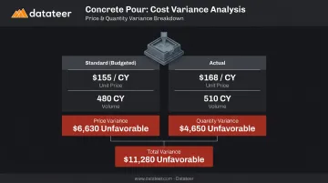
| Price per cubic yard | $155/CY | $168/CY |
| Cubic yards (for scope complete) | 480 CY | 510 CY |
Price Variance Calculation
(Actual Price – Standard Price) × Actual Quantity Purchased = ($168 – $155) × 510 = $13 × 510 = $6,630 Unfavorable
A regional concrete shortage drove actual price $13/CY above standard. That's a procurement issue — the project manager didn't overpour, but the firm paid more per yard than the bid assumed. Result: $6,630 unfavorable, attributed to procurement.
Quantity Variance Calculation
(Actual Quantity Used – Standard Quantity Allowed) × Standard Price = (510 – 480) × $155 = 30 × $155 = $4,650 Unfavorable
The crew poured 30 CY more than the standard allowed, due to subgrade irregularities requiring additional fill. This is a field operations issue — the concrete price was irrelevant here. Using standard price isolates the quantity problem cleanly. Result: $4,650 unfavorable, attributed to field conditions.
Total Variance
$6,630 + $4,650 = $11,280 Unfavorable
Management Response
The variance doesn't just go in a report — it triggers specific actions:
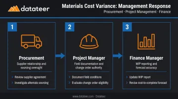
- Procurement reviews the supplier agreement and investigates whether the regional shortage warrants emergency sourcing from an alternate supplier for remaining pours
- Project manager documents the subgrade irregularity and evaluates whether a change order to the owner is warranted — if the condition wasn't in the original scope, the cost may be recoverable
- Construction finance manager notes the $11,280 variance in the WIP report and adjusts the cost-to-complete forecast for remaining foundation work, reflecting the higher-than-standard concrete price
Without decomposing the variance into its two components, none of these targeted responses would be possible.
How Datateer Helps Construction Firms Track Material Variances in Real Time
The formula is straightforward. The hard part is data timing.
Most construction firms are working with materials cost data that's 10–20 days old by the time it reaches a WIP report. By the time an unfavorable price variance on Phase 2 concrete shows up in the monthly close, Phase 3 procurement is already underway. The window to renegotiate, adjust scope, or revise the cost-to-complete has closed.
An Autodesk/FMI study estimated that bad or untimely data cost global construction $1.85 trillion in 2020 — with rework linked to poor data decisions accounting for $88.69 billion of that figure. The cost of delayed variance visibility isn't abstract.
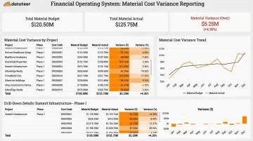
Datateer's Financial Operating System connects directly to 20+ construction ERPs (including Procore, Sage, Viewpoint Vista, and Acumatica) and refreshes WIP and cost dashboards overnight. Construction finance managers can see material cost variances by project, phase, and cost code as they develop — not during the next monthly close.
The platform's Cost Variance Reporting and Material Price Escalation Analytics modules surface:
- Actual vs. budget at job, phase, cost code, and resource type levels
- Trend lines showing whether a job is converging or diverging from target
- Drill-down to source transactions in the ERP for root-cause investigation without switching systems
- Material price escalation compared against bid-estimate unit prices and current PPI and ENR indices
Together, these capabilities close the feedback loop that monthly closes leave open. Instead of discovering a concrete cost overrun after Phase 3 procurement is locked in, a construction finance manager sees the variance flag within days — with enough project timeline remaining to investigate, renegotiate the next order, or revise the cost-to-complete before it threatens final margin.
Both modules are included in Datateer's flat annual pricing, starting at $10,000/year per data source with unlimited users. Implementation takes 2–4 weeks.
Frequently Asked Questions
What is the formula for material cost variance?
Direct materials cost variance = (Actual Quantity × Actual Price) – (Standard Quantity × Standard Price). It decomposes into a price variance component — (Actual Price – Standard Price) × Actual Quantity — and a quantity variance component — (Actual Quantity Used – Standard Quantity Allowed) × Standard Price — that sum to the total.
How do you calculate CV and SV?
In earned value management, Cost Variance (CV) = Earned Value – Actual Cost, and Schedule Variance (SV) = Earned Value – Planned Value. For materials cost control, price variance and quantity variance are more operationally useful — they point directly to procurement decisions and field efficiency, not just aggregate project performance.
What is PPV and how is it calculated?
Purchase Price Variance (PPV) is the same concept as direct materials price variance: (Standard Price – Actual Price) × Actual Quantity Purchased. A positive PPV means you paid less than standard (favorable); a negative PPV means you paid more (unfavorable), with the sign convention reversed from the standard materials price variance formula. Both measure the same underlying gap.
What causes direct materials cost variance on a construction project?
The main drivers are commodity price fluctuations between bid and procurement, emergency or off-contract purchasing, field waste and overpouring, inaccurate quantity take-offs in the original estimate, and scope changes that aren't captured through formal change orders. Price variance and quantity variance will usually point to different root causes within that list.
What is the difference between a favorable and unfavorable material variance?
A favorable variance means actual materials cost came in below the standard — a positive outcome for project margin. An unfavorable variance means actual cost exceeded the standard, signaling a procurement issue, field efficiency problem, or estimating inaccuracy that needs investigation. Even favorable variances deserve review — they can reflect deferred scope rather than genuine savings.
How often should construction firms calculate direct materials cost variance?
At minimum, monthly during active project phases. Ideally, at each billing period or project milestone so corrective actions can influence cost-to-complete. The further into a project phase a variance is discovered, the fewer options remain to address it — automated, near-daily visibility gives you time to act on it. Monthly reviews rarely do.